27 Who rolls the six? Binomial distribution.

Slide 0

Hello and welcome to this new episode. Let’s talk today about binomial distribution and about what it has to do with rolling a “6” on a die.

Slide 1

We will look at random experiments again, specifically these:

We flip a coin.

We roll a die and it lands on a “6” or not.

We draw a ball from an urn with black and red balls.

Argentina and Spain play in the final match of a (hypothetical) soccer world championship.

Robert passes the math test or not.

The air temperature at the summit of the Zugspitze is maximum 4° Celsius today.

What do these random experiments have in common? Not much at first glance. However, a second glance shows that each has two possible results. This clearly applies to all these experiments. It also applies to the soccer world championship because in this case, the victorious team will be determined by a penalty shootout, if necessary. According to the rules, the penalty shootout continues until the match is decided, which admittedly sounds strange from a mathematical perspective. Theoretically, it could go on forever, right? Whatever.

Slide 2

We refer to such a random experiment as a Bernoulli trial.

The definition is quite simple. A random experiment that distinguishes exactly two possible outcomes, “success” and “failure,” is called a Bernoulli trial. Very important: The two outcomes do not need to be equally likely.

Slide 3

Let’s look a little more closely at these examples.

A coin flip has the outcomes “heads” and “tails.” Both outcomes are equally likely, and P(heads) = P(tails) = ½.

If you flip a coin multiple times, you can use a tree diagram with a very simple structure to represent the results. You see it shown here.

Slide 4

If we roll a die, you can differentiate the outcomes “6” and “not 6.” However, the two outcomes are not equally likely. P(6) = 1/6 and P(not 6) = 5/6.

If you conduct this experiment multiple times, you can also use a tree diagram here. Its structure is just as simple as for flipping a coin; we only write the corresponding changed probabilities on the branches.

Slide 5

And how do things look with the thumbtack?

The outcomes are “head” and “side.” The two outcomes have different probabilities and – we have already seen this occasionally – there is not a theoretical value for the probability. However: If P(head) = p, then P(side) = 1 – p.

If you conduct the experiment multiple times, then you can – very clearly – use a tree diagram and label it accordingly.

Slide 6

Let’s consider a cactus flower. And yes, now it will be boring.
The outcomes are “flower” and “no flower.” The two outcomes have different probabilities, and this time there is also no theoretical value. 
However:  If P(flower) = p, then P(no flower) = 1 – p.

If you conduct the experiment multiple times, then you can use a tree diagram for representation here as well.

Slide 7

This has been the same situation again and again. Apparently, it is worth introducing a term for this. This term is the Bernoulli sequence.

If you conduct the same Bernoulli trial n times, you obtain a Bernoulli sequence of length n.

The structure of a Bernoulli sequence with probability of success p is simple and can be described using the tree diagram in the figure.

By the way, this was named after Swiss mathematician Jacob I Bernoulli, a member of the prominent Bernoulli family of mathematicians. He worked in the second half of the 17th century and the beginning of the 18th century. 

Slide 8

What do the probabilities look like in each case? We consider this, represent the outcomes in a table for each trial, and start with flipping a coin. If you flip a coin three times, the probability of flipping “heads” three times or not at all is clearly 1/8 for each outcome. The probability of flipping “heads” once or twice is 3/8 for each outcome.

You can calculate the expected value from this. It is

.

Slide 9

This is what it looks like as a histogram; very clear. We can read the numbers that we just calculated. The probability that “heads” is not flipped at all is 1/8, just the same as the probability that “heads” comes up three times in a row. The probability of flipping “heads” once or twice is 3/8 for each outcome. You can very nicely recognize the symmetry resulting from the limitation to only two possibilities.

Slide 10

Now we’ll examine the Bernoulli trial “rolling a 6 with a die.” If you roll the die three times, the probability that a “6” is rolled three times is exactly   or 1/216. The probability that a “6” is rolled twice is . The probability that a “6” is rolled exactly once is . And finally, there are 125 of 216 cases in which a “6” does not appear at all, which corresponds to a probability of .

We calculate the expected value again. It is

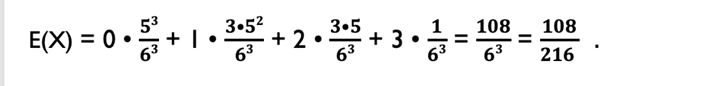
And that is the expected (relative) number of sixes for rolling a die three times.

Slide 11

In this case as well, we look at the outcomes on a histogram.

Slide 12

You can see the general principle even a little better in the example of a thumbtack.

If p is the probability for the outcome “head,” then  is the probability for “head” three times, 𝟑•𝒑² • (𝟏 −𝒑) is the probability for “head” twice, 𝟑•𝒑•(𝟏 −𝒑)² is the probability for “head” one time, and (1-p)³ is the probability that the thumbtack doesn’t land on its head a single time.

Bernoulli trials clearly follow a common “pattern.”

Slide 13

Let’s look at the urn model very generally.

We can simulate a Bernoulli trial by drawing balls from an urn. If we use, for example, black and red balls, then one share (e.g., of the red balls) must correspond to the probability of success p of the actual trial.

A Bernoulli sequence of length n means that you draw a ball at random n times and replace it again.

You can very easily determine the corresponding probabilities – and we have done this in the examples.

Slide 14

Generally speaking: The binomial coefficient  indicates the number of different outcomes that contain exactly k successes (“red balls”) for a Bernoulli sequence of length n (given k from N₀ and k = n).
 
Each outcome with k successes and thus n-k “failures” (“black balls”) has the probability p^k • (1-p)^n-k.

Slide 15

For a Bernoulli sequence of length n and the probability of success p, the probability of exactly k successes (given 0 = k = n) is:

And we have thus reached the starting point for a specific probability distribution, namely for the so-called binomial distribution.

Slide 16

It is defined as follows:

A random variable X is binomially distributed with the parameters n and p if the probability of k successes can be described with a Bernoulli sequence with length n and probability p for a success.  This probability distribution is called binomial distribution B(n;p).

We write (for 0 = k = n): .

When something is generalized in mathematics, it can definitely look a little terrifying at first. Ultimately, though, it shows only what we were able to see relatively easily in the examples. This makes the examples so important. A summary, a definition, or a formula is worthwhile from a mathematical perspective only if there are a sufficient number of examples. Accordingly, they are regularly the beginning of a good mathematical theory. 

Slide 17

Now we will take the last step for today toward a functional recap.

The expected value of a binomially distributed random variable is

  and we can beautifully calculate this as

E(X) = n • p.

Slide 18

Let’s end with an example. We try again to roll a “6.” However, we are not rolling three times, four times, or five times in a row, but this time it will be 50 rolls. Naturally, you can calculate this too, but it is nicer to use a computer for help.

What does the histogram look like now? Noticeably orderly, right? Let’s simply try to understand this qualitatively, at least to some extent. The probabilities are plotted on the Y-axis, and the number of successful attempts on the X-axis. It is unlikely that a “6” will come up 50 times in succession and thus no other number. The probability is  and that is a very small number. It is definitely to be expected that a “6” will appear a few times. But not too often because, after all, there are still five other numbers. Accordingly, it is plausible that – as can be seen here – a “6” will come up between six and ten times for 50 rolls. A lot fewer times and a lot more times is certainly less likely.

There are programs we can use to determine the histograms for (nearly) any p and (nearly) any n. In this example, we used Geogebra. The best thing is for you to look at it yourself and play with the parameters.

We will come back to this again in the next episode.

Slide 19

Many thanks for being here. I look forward to welcoming you again in the next episode.