28 Is Aya somewhat too small for her age? Normal distribution.

Slide 0

I hope you’re all having a great day. Welcome to this new episode in which – as usual – we talk about mathematics. This time we’ll again be talking about a type of probability distribution. This type is normal distribution, an important type of distribution with many interesting applications.

Slide 1

We will start in general with this question:

What is the probability that a random variable will assume particular values?

Let’s first consider what we already know in this context.

A simple example is – as is so often the case – the regular, six-sided die. Each of the results 1, 2, 3, 4, 5, and 6 occurs with an equal probability of p = 1/6. We can view this as equal distribution.

In addition, in the previous episode we looked at binomial distribution and actually got a grasp of it using a formula. Would this perhaps also work with other types of probability distribution? Yes, it is definitely possible. And today is about showing an example of this.

Slide 2

Of course, there are all sorts of (named and unnamed) probability distribution that we certainly can neither consider nor write as a formula. Therefore, in the following slides we will look at only one more example, which is however very important. This is normal distribution and it applies to an entire class of random experiments – just like binomial distribution.

In simple words, our example is: Is Aya somewhat too small for her age?

Slide 3

First, let’s look at normal distribution qualitatively. It is present in many everyday contexts. For instance,

• length
• weight
• head circumference

are normally distributed for newborn babies. And what does this mean? Viewed qualitatively, it is simply: There is a mean value, and the probability is greater that the measured values will be relatively close to this mean value rather than farther away from this mean value.

Slide 4

Let’s consider the height of children. In 2006, the World Health Organization (WHO) published data on this and various other features that were collected in six countries: Brazil, Ghana, India, Norway, Oman, and the United States.

For example, table 27 on page 64 in the corresponding publication contains information on the length of newborn girls. Let’s take a closer look at this table.

Slide 5

Here is an excerpt from the table:

The mean value for the length of girls at birth is 49.1 cm, and the standard deviation (SD) is 1.9 cm. Percentiles are also listed here. Do you remember what percentiles are? These are the numbers in the top row of the table and they indicate percentages. For instance, “75” means that 75 percent of the newborn girls are at most as long as the corresponding value of 50.4 cm.

We will clarify this further on the next slide.

It should be emphasized that the mean value here is the median. It designates the 50 percent mark – and we have frequently used that.

Slide 6

What are percentiles all about?

Let’s assume that Aya, who has just been born, measures 46 cm. Then in terms of length, she would be classified among the lower 5 percent of baby girls.

If she measured 48 cm, then in terms of length, she would rank among the lower 25 percent of baby girls. However, this value would still be within a standard deviation, which was specified as 1.9 cm.

Let’s assume that Aya measures 49 cm. Then in terms of length, she would lie in the middle of baby girls and about half would be bigger and half would be smaller than she is.

And 54 cm? That would be really big because 99 percent of baby girls are born smaller than this Aya.

Slide 7

The deviations from the mean length can now be determined from these values. The symmetry is quite noticeable.

Slide 8

We enter this on a chart. The red bars show the absolute values in the percentiles. In contrast, the blue bars are meant to illustrate the deviation from the median and thus the expected value. Upward and downward deviations are plotted in the same way.

It is all about this deviation. It definitely is not surprising that this deviation exhibits a certain symmetry and that the upward and downward deviations are quite similar for about the same distance from the median.

You can see the Gaussian bell curve – if necessary, using a little imagination.

Slide 9

Let’s look again at the measured values.

The OECD specifies the standard deviation to four decimals points as exactly 1.8627 cm.

If you consider one standard deviation (or more), then you are in the range of up to 47.3 cm and greater than 51.0 cm in length.

If you consider two standard deviations (or more), then you are in the range of up to 45.4 cm and greater than 52.9 cm in length.

Accordingly, you measure one standard deviation or more among fewer than the upper or lower 25 percent of newborn girls. Two standard deviations are a lot more, and fewer than the upper or lower 3 percent of newborn girls fall in this range.

Slide 10

And that characterizes normal distribution.

With normal distribution, 68.3 percent of the data lie within a range determined by the expected value +/- 1 standard deviation.

In the example, therefore, 68.3 percent of the newborns have a length between 47.3 cm and 51.0 cm.

With normal distribution, about 95.5 percent of the data lie within a range determined by the expected value +/- 2 standard deviations.

In the example, therefore, 95.5 percent of the newborns have a length between 45.4 cm and 52.9 cm.

Slide 11

But of course we want to consider the facts more systematically.

If we do that, then we move from binomial distribution to normal distribution. Namely, for large samples, the histograms of binomially distributed random variables can be approximated with bell curves. Do you remember? We saw this in the previous episode for rolling a die 50 times with the outcomes “6” or “not 6” on a histogram.

It really works best using relevant simulations. Bell curves can be described with the term

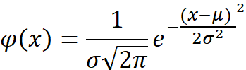
In the term, μ denotes the expected value and σ the standard deviation.

Slide 12

We define the following:

If a random variable with expected value μ and standard deviation σ can be described by the function

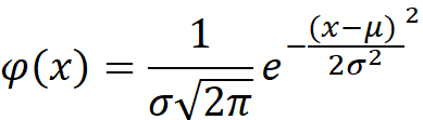
then it is normally distributed. We call this function the probability density.

A random variable is standard normally distributed if the expected value μ = 0 and the standard deviation σ = 1. What you then obtain is the Gaussian bell curve.

Slide 13

Many things in our everyday lives are normally distributed or approximately normally distributed. So you can assume a normal distribution in these cases – and naturally also with a large sample size:

the height and weight of adult persons; students’ performance in the high jump or long jump; the weight of ice cream scoops, packets of tea, bread rolls, and loaves of bread; or the number of gummy bears in a 100 g bag.

In all of these cases, there is a mean value and 50 percent of the measured values lie above it and below it, and most of the measured values lie within a small distance from the mean value. And there are deviations both upwards and downwards.

Slide 14

Thanks for being here today. We’ll meet again in the next episode and talk again about mathematics.